Q-Learning MountainCar
Tabular Q-learning agent solving the classic MountainCar-v0 control problem. The car learns to build momentum by rocking back and forth to reach the goal — a counter-intuitive strategy discovered autonomously through the Bellman equation and epsilon-greedy exploration.
Overview
A reinforcement learning implementation that masters the Gymnasium MountainCar-v0 environment using tabular Q-learning. The challenge: a car starts at the bottom of a valley between two hills, with the goal flag on the right hill. The car's engine is too weak to drive straight up, requiring it to discover the counter-intuitive strategy of rocking back and forth to build momentum — driving up the left hill first before accelerating toward the goal on the right. The agent learns this strategy entirely through trial and error using the Bellman equation: Q(s,a) ← Q(s,a) + α·[r + γ·max Q(s',a') - Q(s,a)]. The continuous state space (position, velocity) is discretized into a 20×20 grid using numpy.digitize, converting infinite observations into a finite Q-table of shape (20, 20, 3) — one entry per (position_bin, velocity_bin, action). Hyperparameters: learning rate α = 0.4, discount factor γ = 0.9, epsilon-greedy exploration with linear decay from ε = 1.0 (pure exploration) to 0.0 (pure exploitation) over all training episodes. The agent starts by taking random actions to explore the state space, gradually shifting to exploit learned Q-values as epsilon decays. Training typically converges after a few thousand episodes, with early failures (reward = -200, time limit exceeded) transitioning to consistent success as the Q-table learns the momentum-building strategy. Includes comprehensive test suite using pytest for unit and integration testing of Q-learning components, training visualization helpers generating reward curves and Q-table heatmaps to diagnose learning progress, and model persistence saving trained Q-tables to Q_table.pkl for evaluation runs. Demonstrates fundamental reinforcement learning concepts: temporal-difference learning propagating future rewards backwards through the Q-table, state discretization balancing granularity vs. sample efficiency, and the exploration-exploitation trade-off critical to discovering non-obvious policies. Perfect for learning RL fundamentals, understanding the Bellman equation in practice, and experimenting with hyperparameter tuning effects on convergence speed and policy quality.
Key Highlights
- ✓Tabular Q-learning with Bellman equation: Q(s,a) ← Q(s,a) + α·[r + γ·max Q(s',a') - Q(s,a)]
- ✓State discretization: continuous (position, velocity) → finite 20×20 grid
- ✓Epsilon-greedy exploration: ε = 1.0 → 0.0 linear decay over training
- ✓Discovers counter-intuitive momentum-building strategy autonomously
- ✓Hyperparameters: learning rate α = 0.4, discount factor γ = 0.9
- ✓Training visualizations: reward curves and Q-table heatmaps
- ✓Comprehensive pytest test suite for RL components
- ✓Model persistence: saves trained Q-table (Q_table.pkl) for evaluation
Technical Deep Dive
The MountainCar Challenge & Counter-Intuitive Strategy
The MountainCar-v0 environment presents a deceptively simple control problem that requires discovering a counter-intuitive solution. The car starts at the bottom of a valley (position ≈ -0.5) between two hills, with the goal flag on the right hill at position +0.5. The catch: the car's engine is too weak to drive straight up the right hill from the valley. The only way to succeed is to rock back and forth, building momentum by first driving up the left hill (negative direction), then accelerating downward to gain speed before ascending the right hill toward the goal. This strategy is completely non-obvious and cannot be learned through simple greedy approaches — the agent must explore seemingly wrong actions (going left when the goal is right) to eventually discover the optimal policy. Q-learning excels at this type of problem because the Bellman equation propagates future rewards backwards, allowing the agent to learn that 'going left' early leads to 'reaching goal' later.
Q-Learning Algorithm & Bellman Equation
The agent implements classic tabular Q-learning using the Bellman equation for temporal-difference updates: Q(s,a) ← Q(s,a) + α·[r + γ·max Q(s',a') - Q(s,a)]. The Q-table maps (position_bin, velocity_bin, action) tuples to expected cumulative rewards, starting with zeros and gradually filling through exploration. At each timestep, the agent observes state s, takes action a, receives reward r, and transitions to next state s'. The TD error [r + γ·max Q(s',a') - Q(s,a)] measures the difference between the estimated value Q(s,a) and the observed value (immediate reward + discounted future value). The learning rate α = 0.4 controls how much the Q-value is adjusted — higher values mean faster learning but more noise, lower values mean slower but more stable convergence. The discount factor γ = 0.9 determines how much future rewards matter — values close to 1 encourage long-term planning (critical for MountainCar where immediate rewards are all -1 until reaching the goal), while lower values favor immediate rewards. Through thousands of episodes, the Q-table converges to represent the optimal policy: from any (position, velocity) state, which action (push left, push right, or no-op) leads to the highest expected future reward.
State Space Discretization & Implementation Details
Gymnasium's MountainCar environment provides continuous observations: position ∈ [-1.2, 0.6] and velocity ∈ [-0.07, 0.07]. Tabular Q-learning requires discrete states, so numpy.digitize maps the infinite state space to a 20×20 grid, creating bins for position and velocity. The Q-table has shape (20, 20, 3) — 20 position bins × 20 velocity bins × 3 actions. A critical implementation detail: np.digitize returns indices in [1, num_bins], but array indexing needs [0, num_bins-1], so the code clips results with np.clip(digitize_result - 1, 0, num_bins - 1) to prevent out-of-bounds errors at state space boundaries. The discretization granularity (20 bins) balances two competing factors: finer discretization (more bins) provides more precise control and better policies but requires more samples to learn each state-action pair; coarser discretization (fewer bins) converges faster but may miss important state distinctions. The 20×20 grid empirically works well for MountainCar, providing sufficient granularity to learn the rocking strategy while keeping the Q-table small enough to learn efficiently.
Exploration vs. Exploitation with Epsilon-Greedy
The epsilon-greedy strategy balances exploring unknown actions (to discover better policies) with exploiting known good actions (to maximize rewards). At each timestep, the agent chooses: with probability ε, take a random action from the action space (exploration); with probability 1-ε, take argmax_a Q(s,a) — the action with highest Q-value (exploitation). The exploration rate ε starts at 1.0 (100% random actions in early episodes) and linearly decays to 0.0 (100% greedy exploitation in final episodes). This schedule is critical for learning: early exploration discovers the counter-intuitive left-hill momentum strategy by randomly trying all actions in all states; mid-training balancing explores variations while exploiting partially learned policies; late-training exploitation refines the policy without wasting episodes on random actions. Without sufficient exploration (e.g., starting at ε=0.5), the agent may never discover that 'going left' leads to success. Without eventual exploitation (e.g., keeping ε=1.0), the agent never converges to a consistent policy. The linear decay schedule (ε = 1.0 - episode/total_episodes) smoothly transitions between these phases.
Training Insights, Visualizations & Testing
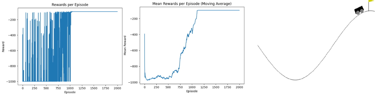
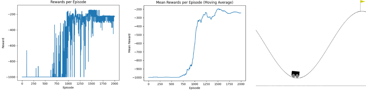
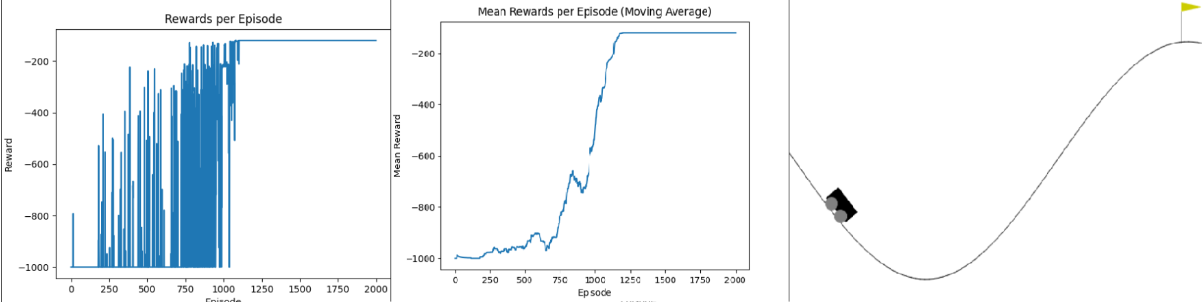
Training typically converges after 2,000-5,000 episodes depending on hyperparameters. Early episodes (ε ≈ 1.0) result in complete failures with reward = -200 (the time limit penalty, as the car never reaches the goal). As the Q-table learns and ε decays, the agent begins discovering the momentum strategy — reward curves show a sharp improvement where the agent first reaches the goal, followed by gradual refinement as it learns to reach the goal faster (rewards approaching -110 to -150, representing the number of steps taken). The code generates three visualization types: (1) Reward curves plotting cumulative reward vs. episode number, showing convergence trends. (2) Q-table heatmaps visualizing the value function across position-velocity state space, revealing higher values (darker colors) near the goal and lower values in the valley. (3) Different starting position evaluations to test policy robustness across the state space. The project includes a comprehensive pytest test suite (car_tests.py) with unit tests for discretization logic, Q-table updates, and epsilon decay, plus integration tests verifying end-to-end training on the Gymnasium environment. Trained models are saved as Q_table.pkl using pickle for later evaluation runs with render=True to visualize the learned policy in action.
Screenshots & Images